2. MOOSE Cookbook

The MOOSE Cookbook contains recipes showing you how to do specific tasks in MOOSE.

2.1. Loading and running models

This section of the documentation explains how to load and run predefined models in MOOSE.

2.1.1. Hello, MOOSE: Load, run and display existing models

helloMoose.main()

This is the Hello MOOSE program. It shows how to get MOOSE to do its most basic operations: to load, run, and graph a model defined in an external model definition file.

The loadModel function is the core of this example. It can accept a range of file and model types, including kkit, cspace and GENESIS .p files. It autodetects the file type and loads in the simulation.

The wildcardFind function finds all objects matching the specified path, in this case Table objects hoding the simulation results. They were all defined in the model file.

2.1.2. The Hodgkin-Huxley demo

This is a self-contained graphical demo implemented by Subhasis Ray, closely based on the ‘Squid’ demo by Mark Nelson which ran in GENESIS.

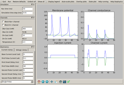
Simulation of Hodgkin-Huxley’s experiment on squid giant axon showing action potentials generated by a step current injection.

The demo has built-in documentation and may be run from the Demos/squid subdirectory of MOOSE. If you want to read a simpler implementation of the same (without the code for setting up GUI), check out hhmodel.

2.1.3. Start, Stop, and setting clocks

startstop.main()

This demo shows how to start, stop, and continue a simulation. This is commonly done when we want to run a model till settling, then change a parameter or deliver a stimulus, and then continue the simulation.

Here, the model is just the output of a PulseGen object which generates periodic pulses. The demo shows how to start the simulation. using the moose.reinit command to reset the model to its initial state, and moose.start command to run the model for the specified duration. We issue multiple moose.start commands and do different things to the model between them. First, we change the delay of the pulseGen. Then we show a number of ways to assign the timestep (dt) to the table object in the simulation. Note that throughout this simulation the pulsegen is going at a uniform rate, it is just being sampled by the output table at different intervals.

2.1.4. Run Python from MOOSE

You can use the PyRun class to run Python statements from MOOSE at runtime. This opens up many possibilities of interleaving computing in Python and MOOSE. You can also use this for debugging simulations.

pyrun.input_output()

The PyRun class can take a double input through trigger field. Whenever another object sends an input to this field, the runString is executed.

The fun part of this is that you can use the input value in your python statements in runString. This is stored in a local variable called input_. You can rename this by setting inputVar field.

Things become even more interesting when you can send out a value computed using Python. PyRun objects allow you to define a local variable called output and whatever value you assign to this, will be sent out through the source field output on successful execution of the runString.

You can rename the output variable by setting outputVar field.

In this example, we send the output of a pulsegen object sending out the values 1, 2, 3 during each pulse and compute the square of these numbers in Python and set output to this square.

The calculated value is assigned to the output variable and in turn sent out to a Table object’s input and gets recorded.

By default PyRun executes the runString whenever a trigger message is received and when its process method is called at each timestep. In both cases it sends out the output value. Since this may cause inaccuracies depending on what the Python statements in runString do, a mode can be specified to disable one of the above. We set mode = 2 to disable the process method. Note that this could also have been done by setting its tick = -1.

mode = 1 will disable trigger message and mode = 0, the default, enables both.

pyrun.run_sequence()

In this example we demonstrate the use of PyRun objects to execute Python statements from MOOSE. Here is a couple of fun things to indicate the power of MOOSE-Python integration.

First we create a PyRun object called Hello. In its initString we put in Python statements that prints the element’s string representation using pymoose-API. When moose.reinit() is called, this causes MOOSE to execute these Python statements which include Python calling a MOOSE function (Python->MOOSE->Python->MOOSE) - isn’t that cool!

We also initialize a counter called hello_count to 0.

The statements in initString gets executed once, when we call moose.reinit().

In the runString we put a couple of print statements to indicate the name fof the object which is running and the current count. Then we increase the count directly.

When we call moose.start(), the runString gets executed at each time step.

The other PyRun object we create, is /World. In its initString apart from ordinary print statements and initialization, we define a Python function called incr_count. This silly little function just increments the global world_count by 1.

The runString for World simply calls this function to increment the count and print it.

We may notice that we assign tick 0 to Hello and tick 1 to World. Looking at the output, you will realize that the sequences of the ticks strictly maintain the sequence of execution.

2.1.5. Accessing and tweaking parameters

tweakingParameters.main()

This example illustrates parameter tweaking. It uses a kinetic model for a relaxation oscillator, defined in kkit format. We use the gsl solver here. The model looks like this:

        _________
        |        |
        V        |
M-----Enzyme---->M*           All in compartment A
|\             /| ^
| \___basal___/   |
|                 |
endo              |
|                 exo
|       _______   |
|       |      \  |
V       V       \ |
M-----Enzyme---->M*           All in compartment B
\             /|
\___basal___/

The way it works: We set the run off for a few seconds with the original model parameters. This version oscillates. Then we double the endo and exo forward rates and run it further to show that the period becomes nearly twice as fast. Then we restore endo and exo, and instead double the initial amounts of M. We run it further again to see what happens. This model takes several seconds to run.

2.1.6. Storing simulation output

Here we’ll show how to store and dump from a table and also using HDF5.

Table can be used for recording and saving data in ascii text formats.

tabledemo.example()

In this example we create a square-pulse generator object and record the output using a table.

The steps are:

1. Create a PulseGen element pulse.
2. Set delay[0]=1.0, width[0]=0.2, level[0]=0.5, so it generates 0.2 s wide square pulses with 0.5 amplitude every 1 s.
3. Create a Table element tab.
4. Connect the outputValue field of pulse to tab.
5. We set tick-interval of ticks 0 and 1 to 0.01 and schedule pulse on tick 0 and tab on tick 1.

5. Run the simulation for 5 s and save data to the ascii file output_tabledemo.csv.

HDF5 is a self-describing file format for storing large datasets. MOOSE has an utility HDF5DataWriter for saving simulations data in HDF5 files.

hdfdemo.example()

In this example

1. We create a passive neuronal compartment comp.
2. We create an HDF5DataWriter object hdfwriter for writing to a file output_hdfdemo.h5. The mode of the HDF5DataWriter is set to 2 which means if a file of the same name exists, it will be overwritten.
3. The membrane voltage Vm and membrane current Im of comp are connected to hdfwriter for recording.
4. We set some attributes of the datasets and the file.
5. We run the simulation, hdfwriter records and stores the Vm and Im values over time.
6. We close the file by calling close() method of hdfwriter.

Running this snippet creates the file output_defdemo.h5 which reflects the structure of the model:

c[0]
|
|___im
|
|___vm

im and vm are datasets containing Im and Vm field values recorded from comp.

2.1.7. Computing arbitrary functions on the fly

Sometimes you want to calculate arbitrary function of the state variables of one or more elements and feed the result into another element during a simulation. The Function class is useful for this.

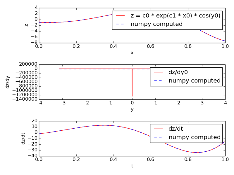
function.example()

Function objects can be used to evaluate expressions with arbitrary number of variables and constants. We can assign expression of the form:

f(c0, c1, ..., cM, x0, x1, ..., xN, y0,..., yP ) 

where ci‘s are constants and xi‘s and yi‘s are variables.

The constants must be defined before setting the expression and variables are connected via messages. The constants can have any name, but the variable names must be of the form x{i} or y{i} where i is increasing integer starting from 0.

The xi‘s are field elements and you have to set their number first (function.x.num = N). Then you can connect any source field sending out double to the ‘input’ destination field of the x[i].

The yi‘s are useful when the required variable is a value field and is not available as a source field. In that case you connect the requestOut source field of the function element to the get{Field} destination field on the target element. The yi‘s are automatically added on connecting. Thus, if you call:

moose.connect(function, 'requestOut', a, 'getSomeField')
moose.connect(function, 'requestOut', b, 'getSomeField')

then a.someField will be assigned to y0 and b.someField will be assigned to y1.

In this example we evaluate the expression: z = c0 * exp(c1 * x0) * cos(y0)

with x0 ranging from -1 to +1 and y0 ranging from -pi to +pi. These values are stored in two stimulus tables called xtab and ytab respectively, so that at each timestep the next values of x0 and y0 are assigned to the function.

Along with the value of the expression itself we also compute its derivative with respect to y0 and its derivative with respect to time (rate). The former uses a five-point stencil for the numerical differentiation and has a glitch at y=0. The latter uses backward difference divided by dt.

Unlike Func class, the number of variables and constants are unlimited in Function and you can set all the variables via messages.

2.1.8. Solving arbitrary differential equations

The Function classes are also useful for setting up arbitrary differential equations. MOOSE supports solution of such equation systems, with the caveat that it thinks they should be chemical systems and therefore interprets the variables as concentrations. MOOSE does not permit the concentrations to go negative.

diffEqSolution.main()

This snippet illustrates the solution of an arbitrary set of differential equations using the Func class and the Pool class. The equations solved here are:

tauI.m' = Ca - Ca_tgt
tauG.chan' = m - chan

These equations are taken from: O’Leary et al Neuron 2014.

Func evaluates an arbitrary function each timestep. Here this function is the rate of change from the equations above. The rate of change is passed to the increment message of the Pool. The numerical integration method is the Exponential Euler method but this will work fine if the rates are slow compared to the simulation timestep.

Conceptually, the idea is that if Ca is greater than the target level, then more mRNA is made, which makes more channels. Although the equations have no upper or lower bounds on m or chan, MOOSE is sensible about preventing the molecular pools from having negative concentrations. This does mean that the solution method employed here won’t work for the general solution of differential equations in non-chemical systems.

This limitation on positive solutions can be overcome with offsets to the variables.

funcRateHarmonicOsc.main()

funcRateHarmonicOsc illustrates the use of function objects to directly define the rates of change of pool concentration. This example shows how to set up a simple harmonic oscillator system of differential equations using the script. In normal use one would prefer to use SBML.

The equations are

p' = v - offset1
v' = -k(p - offset2)

where the rates for Pools p and v are computed using Functions. Note the use of offsets. This is because MOOSE chemical systems cannot have negative concentrations.

The model is set up to run using default Exponential Euler integration, and then using the GSL deterministic solver.

It is also possible to set up other forms of differential equations, where instead of directly controlling the rate of change of a pool, the equations take the form of modifying the rate of a reaction involving a pool.

funcReacLotkaVolterra.main()

The funcReacLotkaVolterra example shows how to use function objects as part of differential equation systems in the framework of the MOOSE kinetic solvers. Here the system is set up explicitly using the scripting, in normal use one would expect to use SBML.

In this example we set up a Lotka-Volterra system. The equations are readily expressed as a pair of reactions each of whose rate is governed by a function:

x' = x( alpha - beta.y )
y' = -y( gamma - delta.x )

This translates into two reactions:

x ---> z        Kf = beta.y - alpha
y ---> z        Kf = gamma - delta.x

Here z is a dummy molecule whose concentration is buffered to zero.

The model first runs using default Exponential Euler integration. This is not particularly accurate even with a small timestep. The model is then converted to use the deterministic Kinetic solver Ksolve. This is accurate and faster. Note that we cannot use the stochastic GSSA solver for this system, it cannot handle a reaction term whose rate keeps changing.

The solutions of such systems are much more accurate and faster using the chemical kinetic solver than with the basic exponential Euler method. However, it is important to point out that the use of arbitrary differential equations to represent chemical systems is discouraged in MOOSE. This is for the simple reason that they are abstractions, frequently with serious flaws, of the underlying chemistry. At the current time the stochastic solver cannot handle systems formulated with functions rather than chemical objects.

2.2. Chemical Signaling models

This section of the documentation explains how to do operations specific to the chemical signaling.

2.2.1. Running with different numerical methods

switchKineticSolvers.main()

At zero order, you can select the solver you want to use within the function moose.loadModel( filename, modelpath, solver ). Having loaded in the model, you can change the solver to use on it. This example illustrates how to assign and change solvers for a kinetic model. This process is necessary in two situations:

• If we want to change the numerical method employed, for example, from deterministic to stochastic.
• If we are already using a solver, and we have changed the reaction network by adding or removing molecules or reactions.

Note that we do not have to change the solvers if the volume or reaction rates change. In this example the model is loaded in with a gsl solver. The sequence of solver calculations is:

1. gsl
2. ee
3. gsl
4. gssa
5. gsl

If you’re removing the solvers, you just delete the stoichiometry object and the associated ksolve/gsolve. Should there be diffusion (a dsolve)then you should delete that too. If you’re building the solvers up again, then you must do the following steps in order:

1. build up the ksolve/gsolve and stoich (any order)
2. Assign stoich.ksolve
3. Assign stoich.path.

See the Reaction-diffusion section should you want to do diffusion as well.

2.2.2. Changing volumes

scaleVolumes.main()

This example illustrates how to run a model at different volumes. The key line is just to set the volume of the compartment:

compt.volume = vol

If everything else is set up correctly, then this change propagates through to all reactions molecules.

For a deterministic reaction one would not see any change in output concentrations. For a stochastic reaction illustrated here, one sees the level of ‘noise’ changing, even though the concentrations are similar up to a point. This example creates a bistable model having two enzymes and a reaction. One of the enzymes is autocatalytic. This model is set up within the script rather than using an external file. The model is set up to run using the GSSA (Gillespie Stocahstic systems algorithim) method in MOOSE.

To run the example, run the script

python scaleVolumes.py

and hit enter every cycle to see the outcome of stochastic calculations at ever smaller volumes, keeping concentrations the same.

2.2.3. Feeding tabulated input to a model

analogStimTable.analogStimTable()

Example of using a StimulusTable as an analog signal source in a reaction system. It could be used similarly to give other analog inputs to a model, such as a current or voltage clamp signal.

This demo creates a StimulusTable and assigns it half a sine wave. Then we assign the start time and period over which to emit the wave. The output of the StimTable is sent to a pool a, which participates in a trivial reaction:

table ----> a <===> b

The output of a and b are recorded in a regular table for plotting.

2.2.4. Finding steady states

findChemSteadyState.getState(ksolve, state)

This function finds a steady state starting from a random initial condition that is consistent with the stoichiometry rules and the original model concentrations.

findChemSteadyState.main()

This example sets up the kinetic solver and steady-state finder, on a bistable model of a chemical system. The model is set up within the script. The algorithm calls the steady-state finder 50 times with different (randomized) initial conditions, as follows:

• Set up the random initial condition that fits the conservation laws
• Run for 2 seconds. This should not be mathematically necessary, but for obscure numerical reasons it makes it much more likely that the steady state solver will succeed in finding a state.
• Find the fixed point
• Print out the fixed point vector and various diagnostics.
• Run for 10 seconds. This is completely unnecessary, and is done here just so that the resultant graph will show what kind of state has been found.

After it does all this, the program runs for 100 more seconds on the last found fixed point (which turns out to be a saddle node), then is hard-switched in the script to the first attractor basin from which it runs for another 100 seconds till it settles there, and then is hard-switched yet again to the second attractor and runs for 400 seconds.

Looking at the output you will see many features of note:

• the first attractor (stable point) and the saddle point (unstable fixed point) are both found quite often. But the second attractor is found just once. It has a very small basin of attraction.
• The values found for each of the fixed points match well with the values found by running the system to steady-state at the end.
• There are a large number of failures to find a fixed point. These are found and reported in the diagnostics. They show up on the plot as cases where the 10-second runs are not flat.

If you wanted to find fixed points in a production model, you would not need to do the 10-second runs, and you would need to eliminate the cases where the state-finder failed. Then you could identify the good points and keep track of how many of each were found.

There is no way to guarantee that all fixed points have been found using this algorithm! If there are points in an obscure corner of state space (as for the singleton second attractor convergence in this example) you may have to iterate very many times to find them.

You may wish to sample concentration space logarithmically rather than linearly.

findChemSteadyState.makeModel()

This function creates a bistable reaction system using explicit MOOSE calls rather than load from a file

2.2.5. Making a dose-response curve

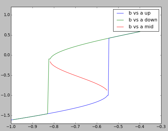
chemDoseResponse.main()

This example builds a dose-response of a bistable model of a chemical system. It uses the kinetic solver Ksolve and the steady-state finder SteadyState. The model is set up within the script.

The basic approach is to increment the control variable, a in this case, while monitoring b. The algorithm marches through a series of values of the buffered pool a and measures resultant values of pool b. At each cycle the algorithm calls the steady-state finder. Since a is incremented only a small amount on each step, each new steady state is (usually) quite close to the previous one. The exception is when there is a state transition.

Here we plot three dose-response curves to illustrate the bistable nature of the system.

On the upward going curve in blue, a starts low. Here, b follows the low arm of the curve and then jumps up to the high value at roughly log( [a] ) = -0.55.

On the downward going curve in green, b follows the high arm of the curve forming a nice hysteretic loop. Eventually b has to fall to the low state at about log( [a] ) = -0.83

Through nasty concentration manipulations, we find the third arm of the curve, which tracks the unstable fixed point. This is in red. We find this arm by setting an initial point close to the unstable fixed point, which the steady-state finder duly locates. We then follow a dose-response curve as with the other arms of the curve.

Note that the steady-state solver doesn’t always succeed in finding a good solution, despite moving only in small steps. Nevertheless the resultant curves are smooth because it gives up pretty close to the correct value, simply because the successive points are close together. Overall, the system is pretty robust despite the core root-finder computations in GSL being temperamental.

In doing a production dose-response series you may wish to sample concentration space logarithmically rather than linearly.

chemDoseResponse.makeModel()

This function creates a bistable reaction system using explicit MOOSE calls rather than load from a file. The reaction is:

a ---b---> 2b    # b catalyzes a to form more of b.
2b ---c---> a    # c catalyzes b to form a.
a <======> 2b    # a interconverts to b.

2.2.6. Building a chemical model from parts

Disclaimer: Avoid doing this for all but the very simplest models. This is error-prone, tedious, and non-portable. For preference use one of the standard model formats like SBML, which MOOSE and many other tools can read and write.

Nevertheless, it is useful to see how these models are set up. There are several tutorials and snippets that build the entire chemical model system using the basic MOOSE calls. The sequence of steps is typically:

1. Create container (chemical compartment) for model. This is typically a CubeMesh, a CylMesh, and if you really know what you are doing, a NeuroMesh.

2. Create the reaction components: pools of molecules moose.Pool; reactions moose.Reac; and enzymes moose.Enz. Note that when creating an enzyme, one must also create a molecule beneath it to serve as the enzyme-substrate complex. Other less-used components include Michaelis-Menten enzymes moose.MMenz, input tables, pulse generators and so on. These are illustrated in other examples.

3. Assign parameters for the components.

   • Compartments have a volume, and each subtype will have quite elaborate options for partitioning the compartment into voxels.
   • Pool s have one key parameter, the initial concentration concInit.
   • Reac tions have two parameters: Kf and Kb.
   • Enz ymes have two primary parameters kcat and Km. That is enough for MMenz ymes. Regular Enz ymes have an additional parameter k2 which by default is set to 4.0 times kcat, but you may also wish to explicitly assign it if you know its value.

4. Connect up the reaction system using moose messaging.

5. Create and connect up input and output tables as needed.

6. Create and connect up the solvers as needed. This has to be done in a specific order. Examples are linked below, but briefly the order is:

   1. Make the compartment and reaction system.
   2. Make the Ksolve or Gsolve.
   3. Make the Stoich.
   4. Assign stoich.compartment to the compartment
   5. Assign stoich.ksolve to either the Ksolve or Gsolve.
   6. Assign stoich.path to finally fill in the reaction system.

   There is an additional step if diffusion is also present, see `Reaction-diffusion in a cylinder`_.

Some examples of doing this are in:

• Making a dose-response curve , which defines a small bistable system including three Pool s, two Enz ymes and a Reac tion.
• Feeding tabulated input to a model, which shows how to connect up a StimulusTable object to a simple 2-molecule reaction.
• `Reaction-diffusion in a cylinder`_, which defines a simple binding reaction and embeds it in a 1-dimensional diffusive volume of a cylinder.

The recommended way to build a chemical model, of course, is to load it in from a file format specific to such models. MOOSE understands SBML, kkit.g (a legacy GENESIS format), and cspace (a very compact format used in a large study of bistables from Ramakrishnan and Bhalla, PLoS Comp. Biol 2008).

One key concept is that in MOOSE the components, messaging, and access to model components is identical regardless of whether the model was built from parts, or loaded in from a file. All that the file loaders do is to use the file to automate the steps above. Thus the model components and their fields are completely accessible from the script even if the model has been loaded from a file. See Accessing and tweaking parameters for an example of this.

2.2.7. Oscillation models

There are several chemical oscillators defined in the Demos/tutorials/ChemkcalOscillators directory. These include:

1. Slow Feedback Oscillator based on a model by Boris Kholdenko

slowFbOsc.main()

This example illustrates loading, and running a kinetic model for a delayed -ve feedback oscillator, defined in kkit format. The model is one by Boris N. Kholodenko from Eur J Biochem. (2000) 267(6):1583-8

This model has a high-gain MAPK stage, whose effects are visible whem one looks at the traces from successive stages in the plots. The upstream pools have small early peaks, and the downstream pools have large delayed ones. The negative feedback step is mediated by a simple binding reaction of the end-product of oscillation with an upstream activator.

We use the gsl solver here. The model already defines some plots and sets the runtime to 4000 seconds. The model does not really play nicely with the GSSA solver, since it involves some really tiny amounts of the MAPKKK.

Things to do with the model:

• Look at model once it is loaded in:

  moose.le( '/model' )
  moose.showfields( '/model/kinetics/MAPK/MAPK' )
  

• Behold the amplification properties of the cascade. Could do this by blocking the feedback step and giving a small pulse input.

• Suggest which parameters you would alter to change the period of the oscillator:

  • Concs of various molecules, for example:

    ras_MAPKKKK = moose.element( '/model/kinetics/MAPK/Ras_dash_MKKKK' )
    moose.showfields( ras_MAPKKKK )
    ras_MAPKKKK.concInit = 1e-5
    

  • Feedback reaction rates

  • Rates of all the enzymes:

    for i in moose.wildcardFind( '/##[ISA=EnzBase]'):
         i.kcat *= 10.0
    

2. Repressilator, based on Elowitz and Liebler, Nature 2000.

repressillator.main()

This example illustrates the classic Repressilator model, based on Elowitz and Liebler, Nature 2000. The model has the basic architecture:

A ---| B---| C
T            |
|            |
|____________|

where A, B, and C are genes whose products repress eachother. The plunger symbol indicates inhibition. The model uses the Gillespie (stochastic) method by default but you can run it using a deterministic method by saying python repressillator.py gsl

Good things to do with this model include:

• Ask what it would take to change period of repressillator:

  • Change inhibitor rates:

    inhib = moose.element( '/model/kinetics/TetR_gene/inhib_reac' )
    moose.showfields( inhib )
    inhib.Kf *= 0.1
    

  • Change degradation rates:

    degrade = moose.element( '/model/kinetics/TetR_gene/TetR_degradation' )
    degrade.Kf *= 10.0
    

• Run in stochastic mode:

  • Change volumes, figure out how many molecules are present:

    lac = moose.element( '/model/kinetics/lac_gene/lac' )
    print lac.n``
    

  • Find when it becomes hopelessly unreliable with small volumes.

3. Relaxation oscillator.

relaxationOsc.main()

This example illustrates a Relaxation Oscillator. This is an oscillator built around a switching reaction, which tends to flip into one or other state and stay there. The relaxation bit comes in because once it is in state 1, a slow (relaxation) process begins which eventually flips it into state 2, and vice versa.

The model is based on Bhalla, Biophys J. 2011. It is defined in kkit format. It uses the deterministic gsl solver by default. You can specify the stochastic Gillespie solver on the command line python relaxationOsc.py gssa

Things to do with the model:

• Figure out what determines its frequency. You could change the initial concentrations of various model entities:

  ma = moose.element( '/model/kinetics/A/M' )
  ma.concInit *= 1.5
  

  Alternatively, you could scale the rates of molecular traffic between the compartments:

  exo = moose.element( '/model/kinetics/exo' )
  endo = moose.element( '/model/kinetics/endo' )
  exo.Kf *= 1.0
  endo.Kf *= 1.0
  

• Play with stochasticity. The standard thing here is to scale the volume up and down:

  compt.volume = 1e-18 
  compt.volume = 1e-20 
  compt.volume = 1e-21 
  

2.2.8. Bistability models

There are several bistable models defined in the Demos/tutorials/ChemkcalBistables directory. These include:

1. MAPK feedback loop model.

mapkFB.main()

This example illustrates loading, and running a kinetic model for a bistable positive feedback system, defined in kkit format. This is based on Bhalla, Ram and Iyengar, Science 2002.

The core of this model is a positive feedback loop comprising of the MAPK cascade, PLA2, and PKC. It receives PDGF and Ca2+ as inputs.

This model is quite a large one and due to some stiffness in its equations, it runs somewhat slowly.

The simulation illustrated here shows how the model starts out in a state of low activity. It is induced to ‘turn on’ when a a PDGF stimulus is given for 400 seconds. After it has settled to the new ‘on’ state, model is made to ‘turn off’ by setting the system calcium levels to zero for a while. This is a somewhat unphysiological manipulation!

2. Simple minimal bistable model, run stochastically at different volumes to illustrate the effects of chemical noise.

scaleVolumes.main()

This example illustrates how to run a model at different volumes. The key line is just to set the volume of the compartment:

compt.volume = vol

If everything else is set up correctly, then this change propagates through to all reactions molecules.

For a deterministic reaction one would not see any change in output concentrations. For a stochastic reaction illustrated here, one sees the level of ‘noise’ changing, even though the concentrations are similar up to a point. This example creates a bistable model having two enzymes and a reaction. One of the enzymes is autocatalytic. This model is set up within the script rather than using an external file. The model is set up to run using the GSSA (Gillespie Stocahstic systems algorithim) method in MOOSE.

To run the example, run the script

python scaleVolumes.py

and hit enter every cycle to see the outcome of stochastic calculations at ever smaller volumes, keeping concentrations the same.

3. Strongly bistable model.

strongBis.main()

This example illustrates loading, and running a kinetic model for a bistable system, defined in kkit format. Defaults to the deterministic gsl method, you can pick the stochastic one by

python filename gssa

The model starts out equally poised between sides b and c. Then there is a small molecular ‘tap’ to push it over to b. Then we apply a moderate push to show that it is now very stably in this state. it takes a strong push to take it over to c. Then it takes a strong push to take it back to b. This is a good model to use as the basis for running stochastically and examining how state stability is affected by changing volume.

2.3. Reaction-diffusion models

The MOOSE design for reaction-diffusion is to specify one or more cellular ‘compartments’, and embed reaction systems in each of them.

A ‘compartment’, in the context of reaction-diffusion, is used in the cellular sense of a biochemically defined, volume restricted subpart of a cell. Many but not all compartments are bounded by a cell membrane, but biochemically the membrane itself may form a compartment. Note that this interpretation differs from that of a ‘compartment’ in detailed electrical models of neurons.

A reaction system can be loaded in from any of the supported MOOSE formats, or built within Python from MOOSE parts.

The computations for such models are done by a set of objects: Stoich, Ksolve and Dsolve. Respectively, these handle the model reactions and stoichiometry matrix, the reaction computations for each voxel, and the diffusion between voxels. The ‘Compartment’ specifies how the model should be spatially discretized.

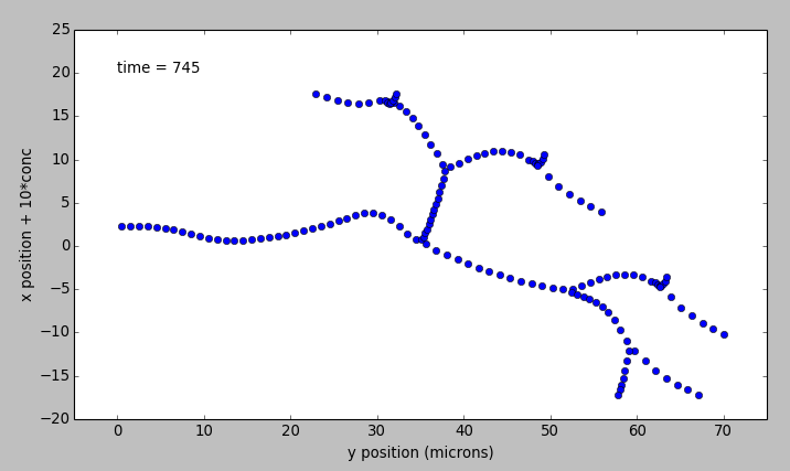
2.3.1. Reaction-diffusion + transport in a tapering cylinder

cylinderDiffusion.makeModel()

This example illustrates how to set up a diffusion/transport model with a simple reaction-diffusion system in a tapering cylinder:

Molecule a diffuses with diffConst of 10e-12 m^2/s.

Molecule b diffuses with diffConst of 5e-12 m^2/s.

Molecule b also undergoes motor transport with a rate of 10e-6 m/s

Thus it ‘piles up’ at the end of the cylinder.

Molecule c does not move: diffConst = 0.0

Molecule d does not move: diffConst = 10.0e-12 but it is buffered.

Because it is buffered, it is treated as non-diffusing.

All molecules other than d start out only in the leftmost (first) voxel, with a concentration of 1 mM. d is present throughout at 0.2 mM, except in the last voxel, where it is at 1.0 mM.

The cylinder has a starting radius of 2 microns, and end radius of 1 micron. So when the molecule undergoing motor transport gets to the narrower end, its concentration goes up.

There is a little reaction in all compartments: b + d <===> c

As there is a high concentration of d in the last compartment, when the molecule b reaches the end of the cylinder, the reaction produces lots of c.

Note that molecule a does not participate in this reaction.

The concentrations of all molecules are displayed in an animation.

2.3.2. A Turing model

TuringOneDim.makeModel()

This example illustrates how to set up a oscillatory Turing pattern in 1-D using reaction diffusion calculations. Reaction system is:

s ---a---> a  // s goes to a, catalyzed by a.
s ---a---> b  // s goes to b, catalyzed by a.
a ---b---> s  // a goes to s, catalyzed by b.
b -------> s  // b is degraded irreversibly to s.

in sum, a has a positive feedback onto itself and also forms b. b has a negative feedback onto a. Finally, the diffusion constant for a is 1/10 that of b.

This chemical system is present in a 1-dimensional (cylindrical) compartment. The entire reaction-diffusion system is set up within the script.

2.3.3. A spatial bistable model

This example illustrates propagation of state flips in a linear 1-dimensional reaction-diffusion system. It uses a bistable system loaded in from a kkit definition file, and places this in a tapering cylinder for pseudo 1-dimentionsional diffusion.

This example illustrates a number of features of reaction-diffusion calculations.

First, it shows how to set up such systems. Key steps are to create the compartment and define its voxelization, then create the Ksolve, Dsolve, and Stoich. Then we assign stoich.compartment, ksolve and dsolve in that order. Finally we assign the path of the Stoich.

For running the model, we start by introducing a small symmetry-breaking increment of concInit of the molecule b in the last compartment on the cylinder. The model starts out with molecules at equal concentrations, so that the system would settle to the unstable fixed point. This symmetry breaking leads to the last compartment moving towards the state with an increased concentration of b, and this effect propagates to all other compartments.

Once the model has settled to the state where b is high throughout, we simply exchange the concentrations of b with c in the left half of the cylinder. This introduces a brief transient at the junction, which soon settles to a smooth crossover.

Finally, as we run the simulation, the tapering geometry comes into play. Since the left hand side has a larger diameter than the right, the state on the left gradually wins over and the transition point slowly moves to the right.

2.3.4. Reaction-diffusion in neurons

Reaction-diffusion systems can easily be embedded into neuronal geometries. MOOSE does so by treating each neuron as a pseudo 1-dimensional object. This means that diffusion only happens along the axis of dendritic segments, not radially from inside to outside a dendrite, nor tangentially around the dendrite circumference. Here we illustrate two cases. The simple case treats the entire neuron as a single, chemically equivalent reaction-diffusion system in a binary branching neuronal tree. The more complex example shows how to set up three chemically distinct kinds of subdivisions within the neuron: the dendritic tree, the dendritic spine heads, and the postsynaptic densities. In both examples we embed a simple Turing-like spatial oscillator in every compartment of the model neurons, so as to see nice oscillations and animations. The first example has a particularly striking pseudo-3D rendition of the neuron and the molecular spatial oscillations within it.

reacDiffBranchingNeuron.main()

reacDiffBranchingNeuron: This example illustrates how to define a kinetic model embedded in the branching pseudo 1-dimensional geometry of a neuron. This means that diffusion only happens along the axis of dendritic segments, not radially from inside to outside a dendrite, nor tangentially around the dendrite circumference. The model oscillates in space and time due to a Turing-like reaction-diffusion mechanism present in all compartments. For the sake of this demo, the initial conditions are set to be slightly different on one of the terminal dendrites, so as to break the symmetry and initiate oscillations. This example uses an external model file to specify a binary branching neuron. This model does not have any spines. The electrical model is used here purely for the geometry and is not part of the computations. In this example we build an identical chemical model throughout the neuronal geometry, using the makeChemModel function. The model is set up to run using the Ksolve for integration and the Dsolve for handling diffusion.

The display has two parts:

1. Animated pseudo-3D plot of neuronal geometry, where each point represents a diffusive voxel and moves in the y-axis to show changes in concentration.
2. Time-series plot that appears after the simulation has ended. The plots are for the first and last diffusive voxel, that is, the soma and the tip of one of the apical dendrites.

reacDiffBranchingNeuron.makeChemModel(compt)

This function sets up a simple oscillatory chemical system within the script. The reaction system is:

s ---a---> a  // s goes to a, catalyzed by a.
s ---a---> b  // s goes to b, catalyzed by a.
a ---b---> s  // a goes to s, catalyzed by b.
b -------> s  // b is degraded irreversibly to s.

in sum, a has a positive feedback onto itself and also forms b. b has a negative feedback onto a. Finally, the diffusion constant for a is 1/10 that of b.

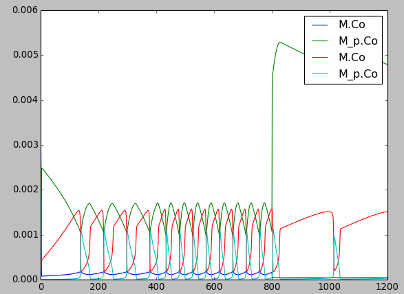
reacDiffSpinyNeuron.main()

This example illustrates how to define a kinetic model embedded in the branching pseudo-1-dimensional geometry of a neuron. The model oscillates in space and time due to a Turing-like reaction-diffusion mechanism present in all compartments. For the sake of this demo, the initial conditions are set up slightly different on the PSD compartments, so as to break the symmetry and initiate oscillations in the spines. This example uses an external electrical model file with basal dendrite and three branches on the apical dendrite. One of those branches has a dozen or so spines. In this example we build an identical model in each compartment, using the makeChemModel function. One could readily define a system with distinct reactions in each compartment. The model is set up to run using the Ksolve for integration and the Dsolve for handling diffusion. The display has four parts:

1. animated line plot of concentration against main compartment#.
2. animated line plot of concentration against spine compartment#.
3. animated line plot of concentration against psd compartment#.
4. time-series plot that appears after the simulation has ended. The plot is for the last (rightmost) compartment.

reacDiffSpinyNeuron.makeChemModel(compt)

This function setus up a simple oscillatory chemical system within the script. The reaction system is:

s ---a---> a  // s goes to a, catalyzed by a.
s ---a---> b  // s goes to b, catalyzed by a.
a ---b---> s  // a goes to s, catalyzed by b.
b -------> s  // b is degraded irreversibly to s.

in sum, a has a positive feedback onto itself and also forms b. b has a negative feedback onto a. Finally, the diffusion constant for a is 1/10 that of b.

2.3.5. Transport in branching dendritic tree

transportBranchingNeuron.main()

transportBranchingNeuron: This example illustrates bidirectional transport embedded in the branching pseudo 1-dimensional geometry of a neuron. This means that diffusion and transport only happen along the axis of dendritic segments, not radially from inside to outside a dendrite, nor tangentially around the dendrite circumference. In this model there is a molecule a starting at the soma, which is transported out to the dendrites. There is another molecule, b, which is initially present at the dendrite tips, and is transported toward the soma. This example uses an external model file to specify a binary branching neuron. This model does not have any spines. The electrical model is used here purely for the geometry and is not part of the computations. In this example we build trival chemical model just having molecules a and b throughout the neuronal geometry, using the makeChemModel function. The model is set up to run using the Ksolve for integration and the Dsolve for handling diffusion.

The display has three parts:

1. Animated pseudo-3D plot of neuronal geometry, where each point represents a diffusive voxel and moves in the y-axis to show changes in concentration of molecule a.
2. Similar animated pseudo-3D plot for molecule b.
3. Time-series plot that appears after the simulation has ended. The plots are for the first and last diffusive voxel, that is, the soma and the tip of one of the apical dendrites.

2.3.6. Cross-compartment reaction systems

Frequently reaction systems span cellular (chemical) compartments. For example, a membrane-bound molecule may be phosphorylated by a cytosolic kinase, using soluble ATP as one of the substrates. Here the membrane and the cytsol are different chemical compartments. MOOSE supports such reactions. The following snippets illustrate cross-compartment chemistry. Note that the interpretation of the rates of enzymes and reactions does depend on which compartment they reside in.

crossComptSimpleReac.main()

This example illustrates a simple cross compartment reaction:

a <===> b <===> c

Here each molecule is in a different compartment. The initial conditions are such that the end conc on all compartments should be 2.0. The time course depends on which compartment the Reac object is embedded in. The cleanest thing numerically and also conceptually is to have both reactions in the same compartment, in this case the middle one (compt1). The initial conditions have a lot of B. The equilibrium with C is fast and so C shoots up and passes B, peaking at about (2.5,9). This is also just about the crossover point. A starts low and slowly climbs up to equilibrate.

If we put reac0 in compt0 and reac1 in compt1, it behaves the same qualitiatively but now the peak is at around (1, 5.2)

This configuration of reactions makes sense from the viewpoint of having the reactions always in the compartment with the smaller volume, which is important if we need to have junctions where many small voxels talk to one big voxel in another compartment.

Note that putting the reacs in other compartments doesn’t work and in some combinations (e.g., reac0 in compt0 and reac1 in compt2) give numerical instability.

crossComptOscillator.main()

This example illustrates loading and running a reaction system that spans two volumes, that is, is in different compartments. It uses a kkit model file. You can tell if it is working if you see nice relaxation oscillations.

crossComptNeuroMesh.main()

This example illustrates how to define a kinetic model embedded in a NeuroMesh, and undergoing cross-compartment reactions. It is completely self-contained and does not use any external model definition files. Normally one uses standard model formats like SBML or kkit to concisely define kinetic and neuronal models. This example creates a simple reaction:

a <==> b <==> c 

in which a, b, and c are in the dendrite, spine head, and PSD respectively. The model is set up to run using the Ksolve for integration. Although a diffusion solver is set up, the diff consts here are set to zero. The display has two parts: Above is a line plot of concentration against compartment#. Below is a time-series plot that appears after # the simulation has ended. The plot is for the last (rightmost) compartment. Concs of a, b, c are plotted for both graphs.

2.4. Single neuron models

Neurons are modelled as equivalent electrical circuits. The morphology of a neuron can be broken into isopotential compartments connected by axial resistances R_a denoting the cytoplasmic resistance. In each compartment, the neuronal membrane is represented as a capacitance C_m with a shunt leak resistance R_m. Electrochemical gradient (due to ion pumps) across the leaky membrane causes a voltage drive E_m, that hyperpolarizes the inside of the cell membrane compared to the outside.

Each voltage dependent ion channel, present on the membrane, is modelled as a voltage dependent conductance G_k with gating kinetics, in series with an electrochemical voltage drive (battery) E_k, across the membrane capacitance C_m, as in the figure below.

---

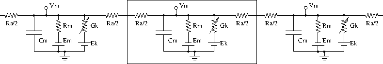
Equivalent circuit of neuronal compartments

---

Neurons fire action potentials / spikes (sharp rise and fall of membrane potential V_m) due to voltage dependent channels. These result in opening of excitatory / inhibitory synaptic channels (conductances with batteries, similar to voltage gated channels) on other connected neurons in the network.

MOOSE can handle large networks of detailed neurons, each with complicated channel dynamics. Further, MOOSE can integrate chemical signalling with electrical activity. Presently, creating and simulating these requires PyMOOSE scripting, but these will be incorporated into the GUI in the future.

To understand channel kinetics and neuronal action potentials, run the Squid Axon demo installed along with MOOSEGUI and consult its help/tutorial.

Read more about compartmental modelling in the first few chapters of the Book of Genesis.

Models can be defined in NeuroML, an XML format which is mostly supported across simulators. Channels, neuronal morphology (compartments), and networks can be specified using various levels of NeuroML, namely ChannelML, MorphML and NetworkML. Importing of cell models in the GENESIS .p format is supported for backwards compatibitility.

2.4.1. Modeling details

Some salient properties of neuronal building blocks in MOOSE are described below. Variables that are updated at every simulation time step are are listed dynamical. Rest are parameters.

• Compartment When you select a compartment, you can view and edit its properties in the right pane. V_m and I_mare plot-able.

  • V_m

    membrane potential (across C_m) in Volts. It is a dynamical variable.

  • C_m

    membrane capacitance in Farads.

  • E_m

    membrane leak potential in Volts due to the electrochemical gradient setup by ion pumps.

  • I_m

    current in Amperes across the membrane via leak resistance R_m.

  • inject

    current in Amperes injected externally into the compartment.

  • initVm

    initial V_m in Volts.

  • R_m

    membrane leak resistance in Ohms due to leaky channels.

  • diameter

    diameter of the compartment in metres.

  • length

    length of the compartment in metres.

• HHChannel

  Hodgkin-Huxley channel with voltage dependent dynamical gates.

  • Gbar

    peak channel conductance in Siemens.

  • E_k

    reversal potential of the channel, due to electrochemical gradient of the ion(s) it allows.

  • G_k

    conductance of the channel in Siemens. G_k(t) = Gbar × X(t)^Xpower × Y(t)^Ypower × Z(t)^Zpower

  • I_k

    current through the channel into the neuron in Amperes.

    I_k(t) = G_k(t) × (E_k-V_m(t))

  • X, Y, Z

    gating variables (range 0.0 to 1.0) that may turn on or off as voltage increases with different time constants.

    dX(t)/dt = X_inf/τ - X(t)/τ

    Here, X_inf and τ are typically sigmoidal/linear/linear-sigmoidal functions of membrane potential V_m, which are described in a ChannelML file and presently not editable from MOOSEGUI. Thus, a gate may open (X_inf(V_m) → 1) or close (X_inf(V_m) → 0) on increasing V_m, with time constant τ(V_m).

  • Xpower, Ypower, Zpower

    powers to which gates are raised in the G_k(t) formula above.

• HHChannel2D The Hodgkin-Huxley channel2D can have the usual voltage dependent dynamical gates, and also gates that depend on voltage and an ionic concentration, as for say Ca-dependent K conductance. It has the properties of HHChannel above, and a few more, similar to in the GENESIS tab2Dchannel reference.

• CaConc This is a pool of Ca ions in each compartment, in a shell volume under the cell membrane. The dynamical Ca concentration increases when Ca channels open, and decays back to resting with a specified time constant τ. Its concentration controls Ca-dependent K channels, etc.

  • Ca

    Ca concentration in the pool in units mM ( i.e., mol/m³).

    d[Ca²⁺]/dt = B × I_Ca - [Ca²⁺]/τ

  • CaBasal/Ca_base

    Base Ca concentration to which the Ca decays

  • tau

    time constant with which the Ca concentration decays to the base Ca level.

  • B

    constant in the [Ca²⁺] equation above.

  • thick

    thickness of the Ca shell within the cell membrane which is used to calculate B (see Chapter 19 of Book of GENESIS.)

2.4.2. Neuronal simulations in MOOSEGUI

Neuronal models in various formats can be loaded and simulated in the MOOSE Graphical User Interface. The GUI displays the neurons in 3D, and allows visual selection and editing of neuronal properties. Plotting and visualization of activity proceeds concurrently with the simulation. Support for creating and editing channels, morphology and networks is planned for the future. MOOSEGUI uses SI units throughout.

2.4.3. Demos

• Cerebellar granule cell

  File -> Load -> ~/moose/Demos/neuroml/GranuleCell/GranuleCell.net.xml

  This is a single compartment Cerebellar granule cell with a variety of channels Maex, R. and De Schutter, E., 1997 (exported from http://www.neuroconstruct.org/). Click on its soma, and See children for its list of channels. Vary the Gbar of these channels to obtain regular firing, adapting and bursty behaviour (may need to increase tau of the Ca pool).

• Pyloric rhythm generator in the stomatogastric ganglion of lobster

  File -> Load -> ~/moose/Demos/neuroml/pyloric/Generated.net.xml

• Purkinje cell

  File -> Load -> ~/moose/Demos/neuroml/PurkinjeCell/Purkinje.net.xml

  This is a purely passive cell, but with extensive morphology [De Schutter, E. and Bower, J. M., 1994] (exported from http://www.neuroconstruct.org/). The channel specifications are in an obsolete ChannelML format which MOOSE does not support.

• Olfactory bulb subnetwork

  File -> Load -> ~/moose/Demos/neuroml/OlfactoryBulb/numgloms2_seed100.0_decimated.xml

  This is a pruned and decimated version of a detailed network model of the Olfactory bulb [Gilra A. and Bhalla U., in preparation] without channels and synaptic connections. We hope to post the ChannelML specifications of the channels and synapses soon.

• All channels cell

  File -> Load -> ~/moose/Demos/neuroml/allChannelsCell/allChannelsCell.net.xml

  This is the Cerebellar granule cell as above, but with loads of channels from various cell types (exported from http://www.neuroconstruct.org/). Play around with the channel properties to see what they do. You can also edit the ChannelML files in ~/moose/Demos/neuroml/allChannelsCell/cells_channels/ to experiment further.

• NeuroML python scripts In directory ~/moose/Demos/neuroml/GranuleCell, you can run python FvsI_Granule98.py which plots firing rate vs injected current for the granule cell. Consult this python script to see how to read in a NeuroML model and to set up simulations. There are ample snippets in ~/moose/Demos/snippets too.

2.4.4. Loading, modifying, saving

2.4.5. Explicit vs. implict methods

2.4.6. Integrate-and-fire models

Simulate current injection into various Integrate and Fire neurons.

All integrate and fire (IF) neurons are subclasses of compartment, so they have all the fields of a passive compartment. Multicompartmental neurons can be created. Even ion channels and synaptic channels can be added to them, say for sub-threshold behaviour.

The key addition is that they have a reset mechanism when the membrane potential Vm crosses a threshold. On each reset, a spikeOut message is generated, and the membrane potential is reset to Vreset. The threshold may be the spike generation threshold as for LIF and AdThreshIF, or it may be the peak of the spike as for QIF, ExIF, AdExIF, and IzhIF. The adaptive IFs have an extra adapting variable apart from membrane potential Vm.

Details of the IFs are given below. The fields of the MOOSE objects are named exactly as the parameters in the equations below.

LIF: Leaky Integrate and Fire:

Rm*Cm * dVm/dt = -(Vm-Em) + Rm*I

QIF: Quadratic LIF:

Rm*Cm * dVm/dt = a0*(Vm-Em)*(Vm-vCritical) + Rm*I

ExIF: Exponential leaky integrate and fire:

Rm*Cm * dVm/dt = -(Vm-Em) + deltaThresh * exp((Vm-thresh)/deltaThresh) + Rm*I

AdExIF: Adaptive Exponential LIF:

Rm*Cm * dVm/dt = -(Vm-Em) + deltaThresh * exp((Vm-thresh)/deltaThresh) + Rm*I - w,

tau_w * dw/dt = a0*(Vm-Em) - w,

At each spike, w -> w + b0 “

AdThreshIF: Adaptive threshold LIF:

Rm*Cm * dVm/dt = -(Vm-Em) + Rm*I,

tauThresh * d threshAdaptive / dt = a0*(Vm-Em) - threshAdaptive,

At each spike, threshAdaptive is increased by threshJump the spiking threshold adapts as thresh + threshAdaptive

IzhIF: Izhikevich:

d Vm /dt = a0 * Vm^2 + b0 * Vm + c0 - u + I/Cm,

d u / dt = a * ( b * Vm - u ),

At each spike, u -> u + d,

By default, a0 = 0.04e6/V/s, b0 = 5e3/s, c0 = 140 V/s are set to SI units, so use SI consistently, or change a0, b0, c0 also if you wish to use other units. Rm from Compartment is not used here, vReset is same as c in the usual formalism. At rest, u0 = b V0, and V0 = ( -(-b0-b) +/- sqrt((b0-b)^2 - 4*a0*c0)) / (2*a0).

IntegrateFireZoo.main()

On the command-line, in Demos/snippets directory, run python IntegrateFireZoo.py. The script will ask you which neuron you want to simulate and you can choose and run what you want. Play with the parameters of the IF neurons in the source code.

2.4.7. The HH model

This is a standalone script for simulating the Hodgkin-Huxley squid axon experiment with a step current injection. The graphical version of the same is The Hodgkin-Huxley demo.

This demo shows how to set the parameters for a Hodgkin-Huxley type ion channel.

Hodgkin-Huxley type ion channels are composed of one or more gates that allow ions to cross the membrane. The gates transition between open and closed states and this, taken over a large population of ion channels over a patch of membrane has first order kinetics, where the rate of change of fraction of open gates (n) is given by:

dn/dt = alpha(Vm) * (1 - n) - beta(Vm) * n

where alpha and beta are rate parameters for gate opening and closing respectively that depend on the membrane potential. The final channel conductance is computed as:

Gbar * m^x * h^y ...

where m, n are the fraction of open gates of different types and x, y are the number of such gates in each channel. We can define the channel by specifying the alpha and beta parameters as functions of membrane potential and the exponents for each gate. The number gates is commonly one or two.

Gate opening/closing rates have the form:

y(x) = (A + B * x) / (C + exp((x + D) / F))

where x is membrane voltage and y is the rate parameter for gate closing or opening.

ionchannel.EREST_ACT = -0.07

Resting membrane potential

ionchannel.K_n_params = [-600.0, -10000.0, -1.0, 0.060000000000000005, -0.01, 125.0, 0.0, 0.0, 0.07, 0.08]

K+ channel in Hodgkin-Huxley model has only one gate, n and these

ionchannel.Na_h_params = [70.0, 0.0, 0.0, 0.07, 0.02, 1000.0, 0.0, 1.0, 0.04000000000000001, -0.01]

Parameters for defining h gate of Na+ channel

ionchannel.Na_m_params = [-4500.000000000001, -100000.0, -1.0, 0.045000000000000005, -0.01, 4000.0, 0.0, 0.0, 0.07, 0.018]

The parameters for defining m as a function of Vm

ionchannel.VDIVS = 3000

Number of divisions in the interpolation table

ionchannel.VMAX = 0.04999999999999999

Maximum x-value for the interpolation table

ionchannel.VMIN = -0.1

We define the rate parameters, which are functions of Vm as interpolation tables looked up by membrane potential. Minimum x-value for the interpolation table

ionchannel.create_1comp_neuron(path, number=1)

Create single-compartmental neuron with Na+ and K+ channels.

Parameters:

path : str

path of the compartment to be created

number : int

number of compartments to be created. If n is greater than 1, we create a vec with that size, each having the same property.

Returns:

comp : moose.Compartment

a compartment vec with number elements.

ionchannel.create_k_proto()

Create and return a K+ channel prototype ‘/library/k’.

The K+ channel conductance has the equation:

g = Gbar * n^4

ionchannel.create_na_proto()

Create and return a Na+ channel prototype ‘/library/na’

The Na+ channel conductance has the equation:

g = Gbar * m^3 * h 

For each gate, we use the HHChannel.setupAlpha function to set up the interpolation table.

ionchannel.current_step_test(simtime, simdt, plotdt)

Create a single compartment and set it up for applying a step current injection.

We use a PulseGen object to generate a 40 ms wide 1 nA current pulse that starts 20 ms after start of simulation.

2.4.8. Analyzing spike trains

2.5. Network models

2.5.1. Connecting two cells via a synapse

Below is the connectivity diagram for setting up a synaptic connection from one neuron to another. The PulseGen object is there for stimulating the presynaptic cell as part of experimental setup. The cells are defined as single-compartments with Hodgkin-Huxley type Na+ and K+ channels (see hhmodel)

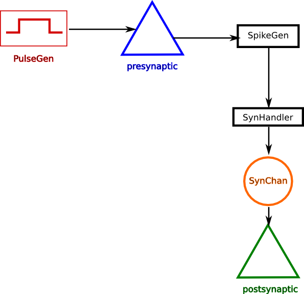
This script demonstrates the use of SynChan class to setup synaptic connection between two single-compartmental Hodgkin-Huxley type neurons.

twocells.create_model()

Create two single compartmental neurons, neuron_A is the presynaptic neuron and neuron_B is the postsynaptic neuron.

1. The presynaptic cell’s Vm is monitored by a SpikeGen object. Whenever the Vm crosses the threshold of the spikegen, it sends out a spike event message.

2. This is event message is received by a SynHandler, which passes the event as activation parameter to a SynChan object.

3. The SynChan, which is connected to the postsynaptic neuron as a channel, updates its conductance based on the activation parameter.

4. The change in conductance due to a spike may evoke an action potential in the post synaptic neuron.

twocells.setup_experiment(presynaptic, postsynaptic, synchan)

Setup step current stimulation of presynaptic neuron. Also setup recording of pre and postsynaptic Vm, Gk of synchan.

2.5.2. Plastic synapse: STDP

Connect two cells via a plastic synapse (STDPSynHandler). Induce spikes spearated by varying intervals, in the pre and post synaptic cells. Plot the synaptic weight change for different intervals between the spike-pairs. This ia a pseudo-STDP protocol and we get the STDP rule.

STDP.main()

On the command-line, in Demos/snippets directory, run python STDP.py

STDP.make_neuron_spike(nrnidx, I=1e-07, duration=0.001)

Inject a brief current pulse to make a neuron spike

STDP.reset_settle()

Call this between every pre-post pair to reset the neurons and make them settle to rest.

STDP.setupModel()

Set up two LIF neurons and connect them by an STDPSynHandler. Set up some tables, and reinit MOOSE before simulation.

2.5.3. Network with Ca-based plasticity

This LIF network with Ca plasticity is based on:

David Higgins, Michael Graupner, Nicolas Brunel Memory Maintenance in Synapses with Calcium-Based Plasticity in the Presence of Background Activity PLOS Computational Biology, 2014.

Author: Aditya Gilra, NCBS, Bangalore, October, 2014.

This uses the Ca-based plasticity rule of:

Graupner, Michael, and Nicolas Brunel. 2012. Calcium-Based Plasticity Model Explains Sensitivity of Synaptic Changes to Spike Pattern, Rate, and Dendritic Location. Proceedings of the National Academy of Sciences, February, 201109359.

The Ca-based bistable synapse has been implemented as the GraupnerBrunel2012CaPlasticitySynHandler class.

class ExcInhNet_HigginsGraupnerBrunel2014.ExcInhNet(J=0.0002, incC=100, fC=0.8, scaleI=4.0, syndelay=0.001, **kwargs)

Recurrent network simulation

Methods

simulate([simtime, dt, plotif])

class ExcInhNet_HigginsGraupnerBrunel2014.ExcInhNetBase(N=1000, fexc=0.8, el=-0.07, vt=-0.05, Rm=20000000.0, Cm=1e-09, vr=-0.06, refrT=0.0, Iinject=5e-10)

Simulates and plots LIF neurons (exc and inh separate).

Methods

simulate([simtime, dt, plotif])

ExcInhNet_HigginsGraupnerBrunel2014.rate_from_spiketrain(spiketimes, fulltime, dt, tau=0.05)

Returns a rate series of spiketimes convolved with a Gaussian kernel; all times must be in SI units.

2.5.4. Providing random input to a cell

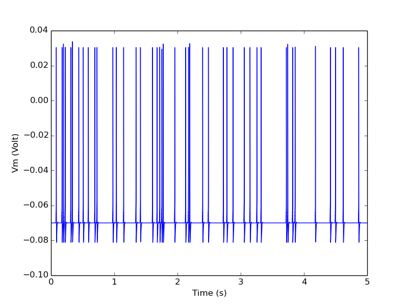
This is an example of simulating random events from a Poisson process and applying the event as spike input to a single-compartmental Hodgekin-Huxley type neuron model.

randomspike.create_cell()

Create a single-compartment Hodgking-Huxley neuron with a synaptic channel.

This uses the ionchannel.create_1comp_neuron() function for model creation.

Returns a dict containing the neuron, the synchan and the synhandler for accessing the synapse,

randomspike.example()

The RandSpike class generates spike events from a Poisson process and sends out a trigger via its spikeOut message. It is very common to approximate the spiking in many neurons as a Poisson process, i.e., the probability of k spikes in any interval t is given by the Poisson distribution:

exp(-ut)(ut)^k/k!

for k = 0, 1, 2, ... u is the rate of spiking (the mean of the Poisson distribution). See wikipedia for details.

Many cortical neuron types spontaneously fire action potentials. These are called ectopic spikes. In this example we simulate this with a RandSpike object with rate 10 spikes/s and send this to a single compartmental neuron via a synapse.

In this model the synaptic conductance is set so high that each incoming spike evokes an action potential.

2.5.5. Recurrent integrate-and-fire network

This LIF network is based on: Ostojic, S. (2014). Two types of asynchronous activity in networks of excitatory and inhibitory spiking neurons. Nat Neurosci 17, 594-600.

Key parameter to change is synaptic coupling J (mV). Critical J is ~ 0.45e-3 V in paper for C/N = 0.1 See what happens for J = 0.2e-3 V versus J = 0.8e-3 V

Author: Aditya Gilra, NCBS, Bangalore, October, 2014.

class ExcInhNet_Ostojic2014_Brunel2000.ExcInhNet(J=0.0008, incC=100, fC=0.8, scaleI=5.0, syndelay=0.0015, **kwargs)

Recurrent network simulation

Methods

simulate([simtime, dt, plotif])

class ExcInhNet_Ostojic2014_Brunel2000.ExcInhNetBase(N=1000, fexc=0.8, el=-0.065, vt=-0.045, Rm=20000000.0, Cm=1e-09, vr=-0.055, refrT=0.0005, Iinject=1.2e-09)

Simulates and plots LIF neurons (exc and inh separate). Author: Aditya Gilra, NCBS, Bangalore, India, October 2014

Methods

simulate([simtime, dt, plotif])

ExcInhNet_Ostojic2014_Brunel2000.rate_from_spiketrain(spiketimes, fulltime, dt, tau=0.05)

Returns a rate series of spiketimes convolved with a Gaussian kernel; all times must be in SI units.

2.5.6. Recurrent integrate-and-fire network with plasticity

2.5.7. A feed-forward network with random input

2.5.8. Using compartmental models in networks

Pyloric rhythm generator in the stomatogastric ganglion of lobster

Stomatogastric ganglion Central Pattern Generator:

generates pyloric rhythm of the lobster

Network model translated from: Prinz, Bucher, Marder, Nature Neuroscience, 2004; STG neuron models translated from: Prinz, Billimoria, Marder, J.Neurophys., 2003.

Translated into MOOSE by Aditya Gilra, Bangalore, 2013, revised 2014.

STG_net.loadRunSTGNeuroML_L123(filename)

Loads and runs the pyloric rhythm generator from NeuroML files.

2.6. Multiscale models

2.6.1. Single-compartment multiscale model

multiscaleOneCompt.main()

This example builds a simple multiscale model involving electrical and chemical signaling, but without spatial dimensions. The electrical cell model is in a single compartment and has voltage-gated channels, including a voltage-gated Ca channel for Ca influx, and a K_A channel which is regulated by the chemical pathways.

The chemical model has calcium activating Calmodulin which activates CaM-Kinase II. The kinase phosphorylates the K_A channel to inactivate it.

The net effect of the multiscale activity is a positive feedback loop where activity increases Ca, which activates the kinase, which reduces K_A, leading to increased excitability of the cell.

In this example this results in a bistable neuron. In the resting state the cell does not fire, but if it is activated by a current pulse the cell will continue to fire even after the current is turned off. Application of an inhibitory current restores the cell to its silent state.

Both the electrical and chemical models are loaded in from model description files, and these files could be replaced if one wished to define different models. However, there are model-specific Adaptor objects needed to map activity between the models of the two kinds. The Adaptors connect specific model entities between the two models. Here one Adaptor connects the electrical Ca_conc object to the chemical Ca pool. The other Adaptor connects the chemical pool representing the K_A channel to its conductance term in the electrical model.

2.6.2. Multi-compartment multiscale model

2.7. Graphics

2.7.1. Displaying time-series plots

2.7.2. Animation of values along an axis

2.7.3. Using MOOGLI widgets to display a neuron